Pre-Lab Assignment: Electron Charge-to-Mass Ratio
This assignment should take approximately 30–45 minutes to complete. You will do this work independently. When you arrive at lab, you will compare your responses with your lab partners and record the outcome of that discussion in your shared lab notebook before beginning the experiment.
Section 1: Context — The Discovery of the Electron
In the late nineteenth century, physicists were puzzled by a phenomenon called cathode rays. When a high voltage was applied across a glass tube from which most of the air had been evacuated, a mysterious ray appeared to emanate from the negative electrode — the cathode. The rays caused the glass at the opposite end of the tube to glow, and they could be deflected by magnets. But what were they? Some physicists believed they were waves, like light. Others believed they were streams of charged particles. The debate lasted decades.
In 1897, J.J. Thomson settled the question. By systematically deflecting cathode rays using both electric and magnetic fields, he showed that the rays consisted of negatively charged particles — particles far lighter than any atom known at the time. He could not measure the charge or mass of these particles separately, but he could measure their ratio: the charge per unit mass, e/m. More remarkably, he found that this ratio was the same regardless of the material of the cathode, the gas in the tube, or the magnitude of the voltage applied. The cathode ray particles — which we now call electrons — were a universal constituent of matter.
This was the first measurement of a subatomic particle. It shattered the prevailing view that atoms were indivisible and laid the foundation for all of modern physics. Thomson’s measurement of e/m was one of the most consequential experiments in the history of science.
Today, the charge-to-mass ratio of the electron is known precisely: e/m = 1.758820 × 10¹¹ C/kg. It is a fundamental constant of nature, and its precise value matters for everything from the design of particle accelerators and electron microscopes to the calibration of mass spectrometers used in medical diagnostics and environmental monitoring.
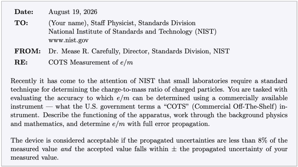
In this experiment you will measure e/m using a method closely related to Thomson’s original approach. Your measurement will be evaluated against a standard set by the National Institute of Standards and Technology (NIST).
Answer the following questions:
- Thomson found that the e/m ratio was the same regardless of the cathode material or gas used in the tube. Why was this result so significant? What did it imply about the nature of the electron?
- Thomson could measure e/m but not e or m individually. Why is measuring a ratio still scientifically useful? What additional measurement would allow you to determine both e and m separately?
Section 2: Instrument Preview
The BroLight BEM-5017 apparatus consists of three main components working together: an electron gun, a pair of Helmholtz coils, and a glass tube containing helium gas at low pressure.
The electron gun: Inside the glass tube, a metal filament (the cathode) is heated by a low-voltage current until it releases electrons through a process called thermionic emission — electrons gain enough thermal energy to escape the metal surface. These electrons are then accelerated through a potential difference V (the accelerating voltage) toward a positively charged anode. The kinetic energy gained by each electron equals the work done by the electric field:
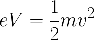
This gives you a beam of electrons with a known, controllable speed.
The Helmholtz coils: Two identical circular coils of wire are mounted coaxially — along the same axis — separated by a distance equal to their radius. This specific geometry produces a remarkably uniform magnetic field in the region between and around the coils. The field is directed along the axis of the coils and is proportional to the current IH passing through them. For this apparatus:
- Coil radius: R = 158 mm
- Number of turns per coil: N = 130
- Magnetic field constant: k = 7.80 × 10⁻⁴ T/A
- Magnetic field: B = kIH
You learned in physics 2 lecture how to derive the magnetic field of a Helmholtz coil from the Biot Savart law. For now, treat B = kIH as a known result. The constant k is determined by the coil geometry and encodes all the information about the radius, number of turns, and geometry of the Helmholtz configuration.
The helium gas: The glass tube contains helium at a precisely controlled low pressure. As electrons travel through the tube, they collide with helium atoms, exciting them to emit a faint blue-green glow. This glow traces the path of the electron beam, making it visible to the naked eye.
The mirrored scale: A mirrored scale is mounted at the back of the apparatus. To measure the radius of the electron beam’s circular path without parallax error, you align the beam with its reflection in the mirror before reading the scale. You will practice this technique in lab.
Safety — High Voltage: The accelerating voltage in this experiment is between 100 and 200 V DC. This is above the threshold for electric shock hazard. Do not touch any bare conductors or terminals while the apparatus is powered. All connections should be made with the power supplies off.
Now answer the following questions:
- The filament must warm up for several minutes before the electron beam appears. Why? What physical process requires this warm-up time?
- The Helmholtz coil configuration produces a more uniform magnetic field than a single coil would. Why does uniformity of the magnetic field matter for this experiment? What would happen to the electron beam path if the field were not uniform?
Section 3: Deriving the Measurement Equation
Your goal is to derive an expression for e/m in terms of quantities you can measure directly: the accelerating voltage V , the Helmholtz coil current IH, and the radius of the electron beam’s circular path r.
Work through the following steps. Show all work. Do not look up the final result — derive it. You will compare your derivation with your partners when you arrive at lab.
Step 1: The magnetic force on a moving electron
An electron moving with speed v through a magnetic field B experiences a Lorentz force. When the velocity and field are perpendicular to each other, this force is:

This force acts perpendicular to the velocity at every point along the electron’s path, producing circular motion.
Step 2: Circular motion and the Lorentz force
For an object moving in a circle of radius r at speed v, Newton’s second law gives a centripetal acceleration directed toward the center. The net force required is:
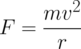
- Set the Lorentz force equal to the centripetal force and solve for v/r. Write your result as an expression for e/m in terms of v, B, and r.
Step 3: Finding the electron’s speed
The electron is accelerated from rest through a potential difference V . The work done on the electron by the electric field equals the kinetic energy it gains.
- Write an equation relating V , e, m, and v using conservation of energy. Then solve this equation for v2.
Step 4: Combining the equations
You now have two equations: one relating e/m to v, B, and r (from Step 2), and one relating v2 to V , e, and m (from Step 3). The speed v appears in both but is not directly measurable.
- Eliminate v between the two equations to find an expression for e/m in terms of V, B, and r only.
- Substitute B = kIH to write your final expression for e/m in terms of V, IH, r, and k only. This is the equation you will use in lab.
- Check your equation dimensionally. Show that the units of your expression for e/m reduce to C/kg. Hint: recall that 1 V = 1 J/C = 1 kg·m2/(A·s3) and that 1 T = 1 kg/(A·s2).
Post-derivation questions:
Now that you have derived the measurement equation, answer these questions:
- For each of the quantities that appear in your derived equation, identify the physical source of uncertainty in measuring it and state whether that uncertainty is primarily systematic or random. Think carefully about how each quantity is actually measured in this experiment before answering.
- Earth’s magnetic field has a magnitude of approximately 5 × 10⁻⁵ T. The Helmholtz coils in this experiment produce fields on the order of 10−3 T. What type of error does Earth’s field introduce — systematic or random? How might you minimize its effect before taking data?
Section 4: Error Propagation Setup and Predictions
In lab you will calculate e/m for each of nine trials and propagate the uncertainty through the full equation. Before you arrive, set up the propagation symbolically so that you can apply it quickly in lab.
- Your equation for e/m involves three measured quantities: V, IH, and r. Each has an associated uncertainty: σV , σIH, and σr. Write the general form of the error propagation equation for e/m. What role does the exponent of each variable play in the propagation? Refer to the error analysis activity if you need to recall the propagation rules for products and powers.
- Explain in your own words why IH and r each contribute a factor of 2 to their relative uncertainty terms, while V contributes only a factor of 1.
- For a typical trial with V ≈ 150 V, IH ≈ 1.5 A, and r ≈ 0.05 m, estimate the relative uncertainty σe/m/(e/m) contributed by each of the three sources. Use these rough estimates for the uncertainties: σV ≈ 2 V, σIH ≈ 0.05 A, σr ≈ 0.002 m. Which source do you predict will contribute most to the total uncertainty?
- The NIST acceptance criterion requires that propagated uncertainties be less than 8% of the measured value. Based on your estimates in question 3, do you expect the apparatus to meet this criterion? What would you need to do differently if the uncertainties were too large?
When you arrive at lab, compare your equation derivations and propagation setups with your lab partners. If your equations differ, work through the physics together before touching the apparatus. Record the outcome of your comparison in your shared lab notebook. Then begin the experiment.
Learning Objective Alignment
Use this table when building your grade proposal to identify which parts of this assignment provide evidence for each learning objective.
| Section / Question | Learning Objectives |
|---|---|
| Section 1, Questions 1–2 | 1, 2 |
| Section 2, Questions 1–2 | 1, 2 |
| Section 3, Questions 1–5 | 1, 5 |
| Post-derivation, Questions 6–7 | 2, 5 |
| Section 4, Questions 1–2 | 5 |
| Section 4, Questions 3–4 | 2, 5, 6 |

