Pre-Lab Assignment:
The Hydrogen Spectrum

This assignment should take approximately 30–45 minutes to complete. You will do this work independently. When you arrive at lab, you will compare your responses with your lab partners and record the outcome of that discussion in your shared lab notebook before beginning the experiment.

Section 1: Context — Reading the Light from Stars

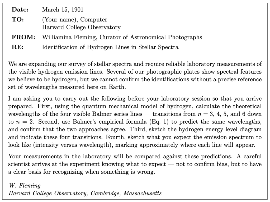
In the 1880s, a woman named Williamina Fleming was hired at the Harvard College Observatory not as an astronomer but as a “computer” — a human calculator paid to classify photographic plates of stellar spectra. She and dozens of women who followed her, including Annie Jump Cannon and Cecilia Payne, spent decades cataloguing the spectra of hundreds of thousands of stars. Their work became the foundation of modern astrophysics.

The key insight that made their cataloguing possible is simple but profound: every element emits and absorbs light at a precise, characteristic set of wavelengths. No two elements produce the same pattern. The spectrum of a star is therefore a kind of fingerprint — a record of every element present in the star’s atmosphere, written in light. By matching the dark absorption lines in a stellar spectrum to the known emission patterns of elements on Earth, astronomers could determine what distant stars are made of without ever leaving the ground.

Hydrogen is the most abundant element in the universe, so its spectral signature appears in nearly every star. The visible hydrogen lines — the Balmer series — were among the first to be characterized. In 1885, Johann Balmer found an empirical formula describing their wavelengths:

where R_H = 1.0974 × 10⁷ m⁻¹ is the Rydberg constant. Balmer had no physical explanation for his formula — it was purely empirical. That explanation came in 1913, when Niels Bohr proposed his model of the hydrogen atom, and more completely from quantum mechanics. In the quantum mechanical picture, the energy levels of hydrogen are:

When an electron transitions from a higher energy level n_i to a lower level n_f , the energy difference is released as a photon:

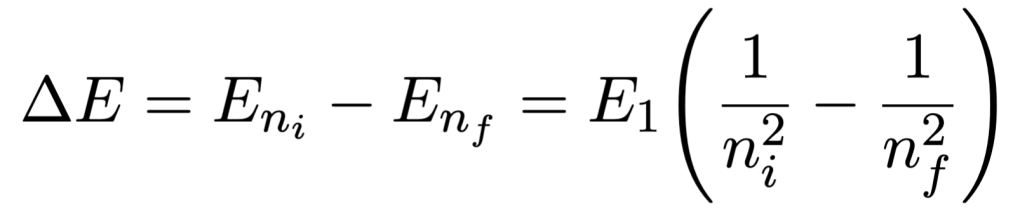
The energy of a photon is related to its wavelength by:

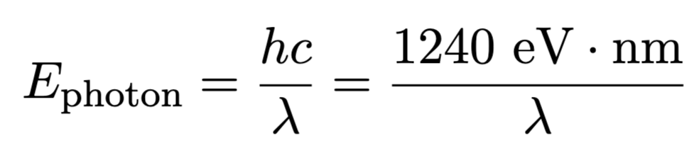
where the combination hc = 1240 eV · nm is convenient for calculations at optical wavelengths.

Before you begin the questions below, take a moment to think about the angle for your public talk flyer. The Balmer series connects laboratory measurements on Earth to the light from distant stars — and the women computers at Harvard were among the first to systematically catalogue those connections. What story do you want to tell about that connection? You will return to this question at the end of the pre-lab.

---

Section 2: The Physics of Emission Spectra

Before you can interpret a spectrum, you need a clear mental model of why spectral lines appear where they do.

1. Why does a hydrogen discharge tube emit light at discrete wavelengths rather than a continuous spectrum? Your answer should connect the structure of the atom to the observation.
2. The Balmer series involves transitions to n_f = 2. Why do transitions to n_f = 1 (the Lyman series) produce ultraviolet photons rather than visible ones? Use the energy level equation to support your answer — do not just state it.
3. In stellar spectra, hydrogen lines appear as dark absorption lines against a bright continuous background, rather than as bright emission lines. Explain the difference between absorption and emission spectra. Why does it make sense that the dark lines in stellar spectra appear at exactly the same wavelengths as the bright hydrogen emission lines?

---

Section 3: Predicting the Balmer Lines

You will now calculate the wavelengths of the four visible Balmer series lines using both the quantum mechanical model and Balmer’s empirical formula. The Balmer series involves transitions from n_i = 3, 4, 5, 6 down to n_f = 2.

Part A: Using the quantum mechanical energy levels

4. For each of the four transitions listed in the table below, calculate ∆E in eV, then calculate the wavelength λ in nm. Identify the color of each line.

Transition (ni → 2)	∆E (eV)	λ (nm)	Color	Series name
3 → 2
4 → 2
5 → 2
6 → 2

Part B: Using Balmer’s empirical formula

5. Use Eq. 1 with R_H = 1.0974 × 10⁷ m⁻¹ to calculate the wavelength for each transition. Show one calculation explicitly (your choice of which transition). Do your two sets of predictions agree? What does this tell you about the relationship between the empirical formula and the quantum mechanical model?

---

Section 4: Predictions

6. Draw an energy level diagram for hydrogen showing at least the first six energy levels (n = 1 through n = 6). Label each level with its quantum number n and its energy in eV. Draw and label arrows showing the four Balmer transitions you calculated above.
7. Sketch the expected emission spectrum (intensity vs. wavelength) across the visible range (roughly 380–700 nm). Mark the approximate position of each Balmer line and label it with the corresponding transition (e.g., 3 → 2). Your sketch does not need to be to scale, but the relative spacing of the lines should be qualitatively correct.

---

Section 5: Instrument Preview

In this lab you will use the Vernier Red Tide spectrometer connected via USB to a computer running Vernier LoggerPro software. A fiber-optic cable carries light from the source to the spectrometer. The instrument contains a diffraction grating and a linear CCD-array detector; LoggerPro displays the measured spectrum as intensity versus wavelength in real time. The grating equation relates the angle θ of a diffraction maximum to the wavelength λ and grating spacing D:

where m is the diffraction order. The spectrometer handles this calculation internally — you will read wavelengths directly from LoggerPro. However, you should understand the underlying physics.

8. In your own words, explain how a diffraction grating separates light of different wavelengths. Why does blue light diffract at a different angle than red light?
9. You will measure both the peak wavelength and the full width at half maximum (FWHM) of each spectral line. Define FWHM. Why does a spectral line have a nonzero width rather than appearing as a perfectly sharp spike? Identify at least one physical reason.
10. The spectrometer has an adjustable integration time (analogous to a camera’s shutter speed). If you increase the integration time, the measured intensity increases. Explain why a very short integration time might cause you to miss faint spectral lines, and why a very long integration time might make bright lines difficult to analyze.

---

Section 6: Thinking About the Public Talk

Your group’s final deliverable for this lab is a one-page public talk flyer — a document you could post to advertise a 20–30 minute talk on atomic spectra and what they reveal about the universe. The flyer should be designed for a general audience with no physics background.

11. What is the core message you want a non-scientist to leave your public talk with? Write 2–3 sentences (not bullet points) that capture the main idea in plain language. This will form the foundation of your flyer’s central claim.
12. The Harvard computers are a compelling human story connected to this science. Write a 2–3 sentence description of their work suitable for a general audience flyer. Avoid jargon.

When you arrive at lab: compare your wavelength predictions (from both methods) with your lab partners and resolve any discrepancies before you begin measurements. Bring your energy level diagram and spectrum sketch — you will refer to them when you see the actual spectrum.

---

Learning Objective Alignment

Use this table when building your grade proposal to identify which parts of this assignment provide evidence for each learning objective.

Section / Question	Learning Objectives
Section 1 (Context)	1, 8
Section 2, Questions 1–3	1, 2
Section 3, Questions 4–5	1, 5
Section 4, Questions 6–7	1, 3
Section 5, Questions 8–10	1, 6
Section 6, Questions 11–12	7, 8