Pre-Lab Assignment: The Photoelectric Effect
Complete this assignment individually before your lab session and submit to D2L before you arrive. When you arrive at lab, your first task is to turn on the mercury lamp so it can warm up. Then compare your derivations and predictions with your lab partners before beginning the experiment.
Section 1: Context — Light as a Particle
In 1887, Heinrich Hertz noticed something puzzling while studying electromagnetic waves. When ultraviolet light fell on a metal surface, the spark produced by his receiver became more vigorous. He did not pursue the observation, but it would not go away. Over the following decade, Wilhelm Hallwachs and Philipp Lenard investigated more carefully, establishing that light caused electrons to be ejected from metal surfaces — a phenomenon they called the photoelectric effect.
What they found was deeply troubling for classical physics. The wave model of light, triumphant since Maxwell’s equations in 1865, predicted that the energy of emitted electrons should increase with the brightness of the light. Instead, Lenard found that the energy of the electrons depended entirely on the color (frequency) of the light — not on its intensity. Increasing the intensity only increased the number of electrons emitted, not their energy. Below a certain threshold frequency, no electrons were emitted at all, no matter how bright the light.
In 1905, Albert Einstein proposed a radical solution. Drawing on Planck’s 1901 theory of quantized oscillators, Einstein suggested that light itself comes in discrete packets of energy — quanta, which we now call photons. Each photon carries energy  , where
  is the frequency and h is Planck’s constant. In the photoelectric effect, one photon is absorbed by one electron. If the photon energy exceeds the energy needed to free the electron from the metal (the work function
  ), the electron escapes with kinetic energy equal to the difference. More intense light means more photons, hence more electrons — but the energy per electron depends only on the frequency.
Einstein’s explanation was elegant, but many physicists were skeptical. Among the most skeptical was Robert Millikan, who spent a decade designing increasingly precise experiments to disprove Einstein’s equation. In 1916, after years of careful stopping potential measurements across multiple spectral lines, Millikan announced his results: Einstein’s equation was confirmed to within experimental error. Millikan received the Nobel Prize in 1923 partly for this work — despite the fact that he never fully accepted Einstein’s photon interpretation.
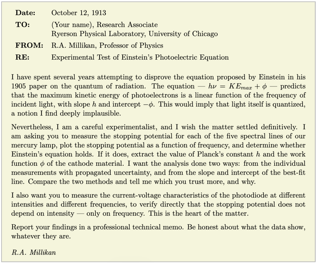
Answer the following questions:
- Lenard found that increasing the intensity of light increased the number of emitted electrons but not their energy. Why is this result impossible to explain with the classical wave model of light, which treats light as a continuous wave carrying energy spread uniformly across its wavefront?
- Einstein’s photon model explains Lenard’s result directly. In your own words, explain why the energy of an emitted photoelectron depends on the frequency of the light but not on its intensity.
- Millikan spent years trying to disprove Einstein’s equation before his own data confirmed it. Why is this kind of adversarial relationship between theory and experiment valuable for science? What would have been lost if Millikan had simply accepted Einstein’s equation without testing it?
Section 2: Instrument Preview
The BroLight BEM-5006 Photoelectric Effect Apparatus consists of four main components working together.
The mercury lamp (BEM-5007): A mercury discharge lamp that emits light at five well-defined spectral lines: 365, 405, 436, 546, and 577 nm. Each wavelength corresponds to a specific electronic transition in mercury atoms. The lamp must warm up for at least 10 minutes before data collection begins — the spectral output is not stable until the lamp reaches operating temperature.
The photodiode enclosure: Contains a vacuum photodiode tube with a metal cathode. When light of sufficient frequency strikes the cathode, photoelectrons are emitted and travel to the anode, producing a measurable photocurrent. The enclosure has two dials on its front:
- Filter wheel: Selects one of five optical filters (365, 405, 436, 546, 577 nm), each transmitting only the corresponding mercury spectral line
- Aperture dial: Selects the diameter of the light beam entering the tube (2 mm, 4 mm, or 8 mm) — changing the aperture changes the intensity of the light without changing its frequency
The DC current amplifier: Measures the extremely small photocurrents produced by the photodiode. It must be zeroed before each measurement session.
The tunable DC power supply: Applies a variable voltage between the anode and cathode of the photodiode tube. By applying a negative (retarding) voltage, you can measure the stopping potential — the voltage at which the photocurrent drops to zero.
Safety — UV Light: The mercury lamp emits ultraviolet radiation at 365 nm. Do not look directly into the lamp when it is on. Keep the protective cap on the lamp enclosure whenever you are not actively collecting data.
Now answer the following questions:
- When you arrive at lab, the first thing you will do is turn on the mercury lamp to begin the warm-up. What will you do during the 10-minute warm-up period? (Refer to the instruction at the top of this pre-lab.)
- The aperture dial changes the intensity of light reaching the photodiode without changing its frequency. Based on Einstein’s photon model, predict what effect changing the aperture will have on: (a) the stopping potential, and (b) the photocurrent when the retarding voltage is zero (the saturation current).
- The current amplifier must be zeroed before measurements begin. If you forgot to zero it and the amplifier read a small nonzero current when no light was present, what type of error would this introduce — systematic or random? Would it affect your measurement of stopping potential, your measurement of photocurrent, or both?
Section 3: Deriving the Measurement Equation
Your central task in this experiment is to measure Planck’s constant h and the work function of the cathode material. To do this you need to connect the physics of the photoelectric effect to the quantities you actually measure in the lab.
Work through the steps below carefully. Show all work and include brief explanations of your reasoning at each step — do not just write equations. Do not look up the final equation. You will compare your derivation with your lab partners when you arrive at lab, and you must agree on the correct form before you begin taking data.
Step 1: Energy of the incoming photon
- For each of the five mercury spectral lines, calculate the photon energy in electron volts (eV). The wavelengths are 365, 405, 436, 546, and 577 nm. Organize your results in a table that also includes the frequency of each line — you will need these frequencies in Section 4.
Step 2: Energy conservation at the cathode surface
When a photon strikes the cathode, it is absorbed by an electron. The electron gains the photon’s full energy  . However, the electron must first do work against the forces holding it inside the metal — it must overcome the work function , the minimum energy required to escape the surface. Any energy left over after escaping becomes kinetic energy of the emitted electron.
- Write an energy conservation equation relating , , and KEmax — the maximum kinetic energy of an emitted photoelectron. Under each term, write a brief phrase explaining what that energy represents physically.
- Your equation involves KEmax — the maximum kinetic energy of the emitted electrons, not the kinetic energy of every electron. Why do some photoelectrons emerge with less than KEmax? What happened to the “missing” energy?
Step 3: Connecting kinetic energy to the stopping potential
In the experiment, you do not measure KEmax directly — you cannot put a speedometer on an electron. Instead, you apply a retarding voltage between the anode and cathode. As the retarding voltage increases, slower electrons are turned back before reaching the anode. At the stopping potential Vstop, even the fastest electrons — those with KEmax — are just barely stopped.
- An electron of charge e moving through a potential difference Vstop gains or loses electrical potential energy. Write an expression for this energy change. Is the electron gaining or losing energy as it moves against the retarding voltage?
- At the stopping potential, the fastest electrons are just barely turned back — they arrive at the anode with zero kinetic energy. Write an energy equation for this condition: the kinetic energy the electron started with equals the electrical potential energy it gave up. Solve this equation to show that: KEmax = eVstop. Explain in words what this equation says: what does eVstop represent physically, and why does it equal KEmax?
Step 4: The measurement equation
- Substitute KEmax = eVstop into your energy conservation equation from Step 2. Rearrange to express Vstop as a linear function of frequency . Your result should have the form: Vstop = A + B where A and B are expressions involving the physical constants h, e, and .
- Identify the slope and y-intercept of your equation. What physical quantity does each one represent? How will you extract h and from a plot of Vstop vs. ?
- Check your equation dimensionally. Verify that the slope A has units of V•s and that the intercept B has units of volts.
Section 4: Predictions and Protocol Design
- Using your derived equation with accepted values of h, e, and = 2.0 eV (a typical work function for the cathode material), calculate the expected stopping potential for each of the five mercury spectral lines. Add these predicted stopping potentials to your table from question 7.
- Sketch a plot of Vstop vs. based on your predictions. Label both axes with units, mark the approximate locations of your five data points, draw the expected best-fit line, and indicate clearly where h/e appears as the slope and where /e appears as the y-intercept.
- Sketch the current-voltage (I-V) curve you expect to observe for a single spectral line. Label the stopping potential Vstop, the region where current increases with voltage, and the saturation current Isat. Then sketch what happens to the curve when: (a) you increase the aperture size (higher intensity) at the same frequency, and (b) you use a higher-frequency spectral line at the same aperture setting.
- Write a brief protocol for how you will carry out the stopping potential measurements for all five wavelengths. Your protocol should address: in what order you will take measurements, how you will determine when the photocurrent is exactly zero, how you will estimate the uncertainty in each stopping potential reading, and how you will organize your data. Your protocol should be clear enough that your lab partner could follow it. You will explain your protocol to your instructor before beginning the experiment — be prepared to defend your choices.
When you arrive at lab: turn on the mercury lamp immediately so it can warm up. Then compare your derivations, predictions, and planned protocols with your lab partners and record the outcome of your discussion in your shared lab notebook. Before you touch any measurement controls, explain your planned protocol to your instructor and get approval to proceed.
Learning Objective Alignment
Use this table when building your grade proposal to identify which parts of this assignment provide evidence for each learning objective.
| Section / Question | Learning Objectives |
|---|---|
| Section 1, Questions 1-2 | 1, 2 |
| Section 1, Question 3 | 2, 8 |
| Section 2, Questions 4–6 | 1, 2 |
| Section 3, Questions 7-14 | 1, 5 |
| Section 4, Questions 15-17 | 3, 6 |
| Section 4, Question 18 | 3 |

