Error Analysis and Propagation of Errors

Opening Scenarios

Your group has been assigned one of the four scenarios below. Read your scenario carefully and work through the discussion questions together. Record your reasoning in your shared lab notebook in your font color. After approximately 20–25 minutes your instructor will bring the class together to discuss what each group found.

Scenario 1: The Recalled Thermometer

Scenario 2: The Mayor’s Press Conference

Scenario 3: The Doctor’s Scale

Scenario 4: A New Measurement of the Proton’s Charge

---

Part 1: Types of Error — A Vocabulary for What You Just Discovered

Learning objectives: 2, 5

In your group discussion you encountered three fundamentally different kinds of error. Here is the vocabulary that scientists use to describe what you observed:

Blunders are mistakes made by the experimenter — misreading an instrument, recording the wrong number, using the wrong units. In Scenario 3, if the doctor had accidentally written 91 kg instead of 90 kg, that would be a blunder. Blunders should be caught and corrected, not reported as a source of error.

Why this matters: You will never write “human error” as a source of error in this course — that is equivalent to saying you made a mistake and left it in. If you suspect a blunder, repeat the measurement.

Systematic error is consistent and directional — it pushes every measurement too high or too low by a predictable amount. In Scenario 1, the thermometers always read 0.8°F too low. No matter how many times you measured the same patient, you would never detect this error by repetition alone — you would just get the same wrong answer more precisely. Systematic errors come from miscalibrated instruments, flawed experimental design, or physical effects that consistently bias the measurement in one direction. Careful experimental design can reveal and correct for them.

Random error causes measurements to fluctuate above and below the true value unpredictably. In Scenario 3, the clinic scale’s uncertainty of ±1.5 kg reflects random error — the reading varies depending on exactly how the patient stands, small vibrations in the floor, rounding in the display. Unlike systematic error, random error can be reduced by taking many measurements and averaging them. However, as you saw in Scenario 3, averaging only helps if your instrument is precise enough to detect the difference you care about in the first place.

The distinction between systematic and random error matters for every experiment you will do this semester. When you identify and articulate the limitations of your experimental setup — as you will do in every pre-lab and every report — you will need to think carefully about which type of error is present and what can be done about it.

---

Station Instructions

At each station you will find an instrument and something to measure. Work through the questions in order — they are designed to guide your thinking. Record everything in your shared lab notebook in your font color, including your reasoning, not just your answers.

Station 1: Length Measurement

Station 2: Current Measurement

Station 3: Period of a Pendulum

Station 4: Angle Measurement and the Hydrogen Spectrum

---

Part 2: Statistical Analysis of Repeated Measurements

Learning objectives: 5, 6

At Station 3 you collected two sets of pendulum period measurements and noticed that your values varied from trial to trial. You also asked whether the two data sets — small displacement and large displacement — are distinguishable. You now have the tools to answer that question, but first you need to learn how to characterize the spread in your data mathematically.

The approach you will use is to repeat a measurement many times, find the average value, and then quantify how much the individual measurements vary around that average. This is how scientists handle random error.

Part A: Setting up your spreadsheet

Open Excel (or your preferred spreadsheet tool). You are going to build the calculation from scratch before using any built-in functions. This is important — you need to understand what the calculation is doing, not just trust a number a computer produces.

Enter your 8 period measurements from the small displacement data set into a single column. Label it clearly.

Part B: Finding the mean

1. The mean (average) value of your measurements is defined as:

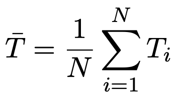
In words: add up all your values and divide by the number of measurements. In Excel, do this manually — use a SUM formula divided by the count. Do not use the AVERAGE function yet.

2. Record your mean value. What does this number represent physically — what is your best estimate of the true period?

Part C: Finding the standard deviation of the observation

The mean tells you your best estimate of the true value. But how spread out are your measurements around that mean? The standard deviation of the observation, σ_T , measures this spread:

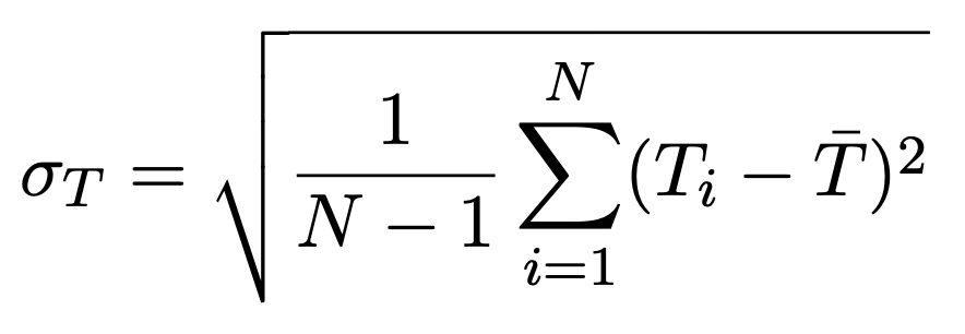
Build this calculation in Excel step by step:

3. Make a second column that contains the difference between each measurement and the mean: 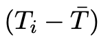. Label this column clearly.
4. Make a third column that contains the square of each of those differences: 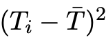. Label it.
5. Sum all the values in the third column and put the result in a single cell below that column.
6. Divide that sum by (N−1), where N is the number of measurements. Put the result in the next cell.
7. Take the square root of that value. This is your standard deviation of the observation, σ_T. Label its cell clearly.
8. Now verify your result using Excel’s built-in function. Type =STDEV() and select your original data column. Does it match your manual calculation? Which standard deviation is Excel reporting — of the observation or of the mean? How do you know?
9. What does σ_T tell you physically? If σ_T is large, what does that mean about your measurements? If it is small?

Part D: Finding the standard deviation of the mean

The standard deviation of the observation tells you how spread out your individual measurements are. But what you really want to know is: how confident are you in your average value? This is captured by the standard deviation of the mean, also called the standard error, σ_m:

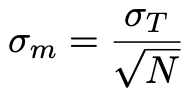
10. Calculate σ_m for your small displacement data set. Record it.
11. This is the value you report as the uncertainty in your measurement of the period. Write your result in the form 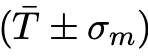with appropriate units.
12. Notice that σ_m depends on N — the number of measurements. What happens to σ_m as you take more measurements? Does doubling the number of measurements halve the uncertainty? What does this tell you about the effort required to significantly reduce your uncertainty?

Part E: Answering the pendulum question

At Station 3 you were asked whether the periods at small and large displacement are distinguishable. You now have the tools to answer this rigorously — but you need to do the analysis for the second data set yourself first.

13. Repeat the full analysis from Parts B, C, and D for your large displacement data set. Record the mean, standard deviation of the observation, standard deviation of the mean, and write your result in the form .
14. Now compare your two results:
    • What is the difference between the two mean values?
    • What are the uncertainties in each mean?
    • Do the two measurements overlap within their uncertainties?
15. Based on your analysis, are the two periods distinguishable? State your conclusion clearly and support it with your numbers. Does your conclusion match your intuition from Station 3?
16. In Physics 1 you discussed this same question. How does having the statistical tools change the way you can answer it compared to then?

---

Part 3: Reporting Results

Learning objectives: 5, 6

You have made several measurements today and calculated uncertainties for each. Before you can use these numbers for anything — a report, a presentation, a comparison to theory — you need to report them correctly. How you round and present a result is not cosmetic.

Why this matters: Every digit you write makes a claim about your confidence in that number. Writing too many digits claims more precision than you have. Writing too few throws away information you worked hard to get.

Rule 1: Round the uncertainty first

Round the uncertainty to 1 significant figure. Exception: if the leading digit of the uncertainty is 1, keep 2 significant figures.

Why the exception? If your uncertainty is 0.19 cm and you round to 1 significant figure you get 0.2 cm — you have just increased your stated uncertainty by 5%. That is a significant distortion. Keeping 2 significant figures when the leading digit is 1 avoids this.

Example: You calculate an uncertainty of 0.386 cm. The leading digit is 3, so round to 1 significant figure: ∆x = 0.4 cm. You calculate an uncertainty of 0.153 cm. The leading digit is 1, so keep 2 significant figures: ∆x = 0.15 cm.

Rule 2: Round the measurement to match the uncertainty

After rounding the uncertainty, round the measurement so it has the same number of decimal places as the rounded uncertainty. The measurement and uncertainty must agree in their last decimal place.

Example: Your measurement is 15.4739 cm and your rounded uncertainty is 0.4 cm. Round the measurement to one decimal place: x = 15.5 cm. Report as: (15.5 ± 0.4) cm.

Your measurement is 8.3471 s and your rounded uncertainty is 0.15 s. Round the measurement to two decimal places: t = 8.35 s. Report as: (8.35 ± 0.15) s.

Rule 3: Write the result in correct form

Put the measurement and uncertainty together in parentheses with the unit outside:

(measurement ± uncertainty) unit

Never write the unit inside the parentheses or attach it to only one of the two numbers.

Example:

• Correct: (15.5 ±0.4) cm
• Incorrect: 15.5 ±0.4 cm
• Incorrect: (15.5 cm ±0.4 cm)
• Incorrect: 15.5 cm ±0.4

Rule 4: In scientific notation, use the same power of ten for both the measurement and the uncertainty

Example: Your result is x = 1.43 × 10⁶ m and your uncertainty is ∆x = 2 × 10⁴ m.

Express both with the same power of ten:

(1.43 ± 0.02) × 10⁶ m

Do not write: (1.43 × 10⁶ ± 2 × 10⁴) m

This second form is technically correct but makes the range of values very hard to read at a glance.

---

Part A: Reporting your station measurements

Apply all four rules to your own measurements. For each result write your answer in correct form and justify your rounding in a few words. Every digit you write must have a reason.

1. Your ruler measurement from Station 1.
   • Write your result in correct form.
   • Justify your rounding: why did you round to this number of decimal places?
2. Your caliper measurement from Station 1.
   • Write your result in correct form.
   • Justify your rounding.
3. Your analog ammeter measurement from Station 2.
   • Write your result in correct form.
   • Justify your rounding.
4. Your digital multimeter measurement from Station 2.
   • Write your result in correct form.
   • Justify your rounding.
5. Your period measurement from Station 3 — use your result from Part 2 in the form .
   • Write your result in correct form.
   • Justify your rounding. Note: σ_m may have more decimal places than you expect — apply the rules carefully.
6. Your angle measurement from Station 4.
   • Write your result in correct form.
   • Justify your rounding.

Part B: Every number matters

Look back at the results you just wrote. For each one ask yourself: does every digit I wrote down mean something? Does my uncertainty honestly reflect what I know about this measurement? If you find a result where the answer is no — fix it now before moving on.

---

Part 4: Propagation of Errors

Learning objectives: 5, 6

You now have measurements with uncertainties, reported in correct form. But in science you rarely stop at a measurement — you use it to calculate something else. When you do, the uncertainty in your measurement carries through into the uncertainty in your result. This is called propagation of errors.

The guiding principle is this: if your measurement could be slightly off from the true value, your calculated result will also be slightly off. Propagation of errors is the mathematical tool that tells you by how much — and more importantly, which measurements contribute most to the uncertainty in your final result.

A note on notation

Throughout this section we use the following symbols:

∆x — the absolute uncertainty in a measurement x. This is the uncertainty you have been calculating and reporting since the stations. It has the same units as x.

∆x/x — the relative uncertainty in a measurement x. This is the absolute uncertainty divided by the measurement itself. It has no units — it tells you the uncertainty as a fraction of the measurement. A relative uncertainty of 0.02 means your measurement is uncertain by about 2%.

Why this matters: Relative uncertainty is useful because it allows you to compare the precision of measurements that have different units or different magnitudes.

When you propagate errors through a multiplication or division, you work with relative uncertainties. When you propagate errors through addition or subtraction, you work with absolute uncertainties. The rules below will tell you which to use and when.

Rule 1: Multiplication and Division

If your result z is calculated by multiplying or dividing measured quantities x and y:

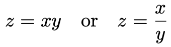
Then the relative uncertainty in z is:

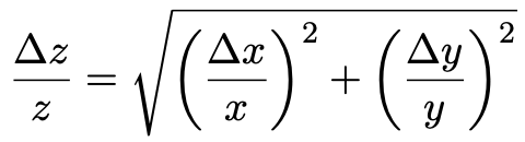
To find the actual uncertainty in z, multiply both sides by z:

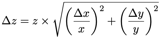
Example: You measure the width of a table as w = (45.2 ± 0.4) cm and its length as l = (122.6 ± 0.5) cm. You want to calculate the area A = wl.

First calculate A:

Then propagate:

Report as: A = (5540 ± 50) cm²

Rule 2: Powers

If your result z involves a measurement x raised to a power n:

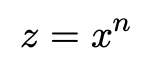
Then:

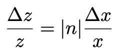
Example: You measure the side of a cube as s = (3.42 ± 0.06) cm and want to calculate the volume V = s³.

Report as: V = (40.0 ± 2.1) cm³.

Rule 3: Trigonometric Functions

For a function like z= sin(x), there is no simple relative uncertainty formula. Instead, you estimate the uncertainty by calculating the difference between the largest possible value of z and the best estimate of z:

Note: the uncertainty in the angle must be in radians for this calculation.

Example: You measure an angle as θ = (35 ± 2)° = (0.611 ± 0.035) rad.

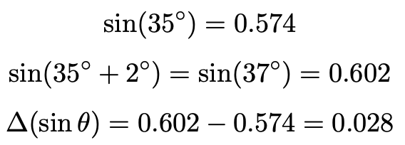
Report as: sin θ = (0.574 ± 0.028) rad

---

Part A: Propagation using your Station 1 measurements

Part B: Propagation using your Station 2 measurements

Part C: Propagation using your Station 4 measurements

---

Part 5: Comparing Results to Theory

Learning objectives: 2, 5, 6

You have calculated the wavelength of the red hydrogen emission line from your own measurement and propagated your uncertainty through the calculation. Now comes the moment that matters in every experiment: does your result agree with what theory predicts?

In science, comparing a measured result to a known or theoretical value is not simply a matter of checking whether two numbers match. Two results agree if they are consistent within their uncertainties — that is, if the known value could plausibly be the true value given the range your measurement allows.

The rule for comparing a result to a known value

Your measured result is reported as (x ± ∆x). The known value is x_known. Your result agrees with the known value if x_known falls within two uncertainties of your measured value — that is, if:

If this condition is met, your result is consistent with the known value. If it is not met, your result is in tension with the known value and you need to think carefully about why.

Why this matters: This is how scientists evaluate whether an experiment worked — not by checking if numbers match exactly, but by asking whether the known value is consistent with the range the measurement allows. An exact match is not required and is actually suspicious — it may suggest the data was manipulated.

Example: A student measures the density of aluminum as (2.58 ± 0.08) g/cm³. The known value is 2.70 g/cm³.

|2.58 − 2.70| = 0.12 g/cm³

2∆x = 2(0.08) = 0.16 g/cm³

Since 0.12 ≤ 0.16, the result is consistent with the known value.

Part A: Comparing your wavelength to the known value

1. Look up the wavelength of the red hydrogen emission line (the Balmer alpha line) from a reliable source. Record the value and cite your source.
2. Apply the comparison rule to your result from Part 4. Show all steps.
3. Does your result agree with the known value? State your conclusion clearly and support it with your numbers.

If your result agrees:

4. Your measurement is consistent with the known value — but that does not mean your experiment was perfect. Look back at your angle measurement and your uncertainty. What are the main limitations of your experimental setup that prevented you from getting a more precise result? What would you change if you repeated this measurement?

If your result does not agree:

5. Your result is in tension with the known value. This does not necessarily mean you made a mistake — it means something in your experiment introduced an error larger than your estimated uncertainty. Work through the following:
   • Look back at your ILE for the angle measurement. Was your estimated uncertainty realistic, or could the true uncertainty be larger than you thought?
   • Could there be a source of systematic error in the spectrometer that you did not account for? What might it be?
   • Could there be a source of random error larger than your ILE that you did not capture?
   • Given your analysis, what do you think is the most likely explanation for the disagreement?

6. Regardless of whether your result agreed or not: what would you need to change about your experimental setup or protocol to increase your confidence in the result?
7. Look back at Scenario 4 from the opening of this activity. A research team reported a measurement of the elementary charge that was in tension with the accepted value. Having now worked through your own comparison, do you think the journalist’s headline — “results conflict with established physics” — was justified? Has your thinking changed from your earlier discussion?